Gravity Terrain Correction

The gravity field measured in areas with topographic relief includes contributions from the surrounding terrain mass. The Seequent Evo Terrain Correction Service (ETCS) corrects for this terrain gravity. Assuming a constant terrain density, ETCS effectively "levels" the surrounding terrain, approximating a situation where all ground has the same elevation as that beneath the station. The ETCS is based on a geometric prism discretization of terrain and applies to ground, airborne, and marine gravity surveys alike.

Definition

Assume a gravity station is located at some location $(x_0, y_0, z_0 + h)$. $z_0$ is assumed to be the topography directly beneath the station, and $h$ is the station height above ground.

A typical gravity processing workflow involves (among other corrections) applying a Bouguer correction to the observed gravity value $g_{obs}$ to account for mass between the station and a reference level (e.g., sea level). The Bouguer correction typically assumes a simple infinite horizontal plate of thickness $z_0$ and a terrain density $\rho$:

$\Delta g_{BA}=2\pi G\rho z_0$

Where $G$ is the gravitational constant. For settings with significant topographic relief, this is a simplification of the actual terrain mass distribution. For example, the mass of a mountain range next to and above the station topography is not accounted for in the Bouguer plate approximation. Similarly, a valley next to and below the station topography represents a mass deficit where the Bouguer plate approximation assumes there is mass. The terrain correction aims to account for these differences by estimating the gravity contribution from the actual terrain mass that differs from the Bouguer plate approximation.

Notice that for gravity stations above ground level $(h>0)$, the terrain correction is here defined consistently with a Bouguer correction plate thickness of $z_0$, i.e. the height of the ground beneath the station. An alternative terrain correction definition (e.g. Nowell, 1999) could be associated with a Bouguer plate thickness corresponding to the total height from sealevel to station ($h+z_0$). However, in either cases, the combined (total) correction (Bouguer + terrain correction) should be the same.

For two-layer situations, where e.g. a layer of water lies on top of the solid earth, a terrain correction can be defined similarly: If a station is above land, at $(x_0, y_0, z_0 + h)$, and assuming a Bouguer correction $\Delta g_{BA}=2\pi G\rho z_0$, the terrain correction involving neighboring water bodies acts to correct for the implicit assumption that all neighboring terrain is similar to that below the station. E.g. a lake within the volume of the corresponding Bouguer correction plate would be corrected for by 'replacing' the solid rock part of the plate with water of a different density ($\rho_w$). A water body above the Bouguer plate would be corrected by 'replacing' water with 'air'.

For stations on or above a water body with surface below or at sea level, the terrain correction is here defined in accord with a Bouguer correction that acts to 'replace' water with solid rock: If a station is located at elevation $h$ above sea level where water column thickness is $d$, a marine Bouguer correction could be defined as $\Delta g_{BA(\text{marine})}=2\pi G(\rho_w-\rho)d$. The corresponding terrain correction similarly acts to remove the gravity contribution from any differences between the actual neighboring stratigraphy and that implied by the Bouguer plate.

Examples illustrating some of the abovementioned corrections are shown further below.

Method

The terrain correction method employed by the ETCS approximates terrain gravity by modeling the relief surrounding a station as a number of rectangular prisms. The gravity field of each of these prisms can be calculated analytically and added together to determine the total contribution at the station location.

Each prism can be thought of as a column of mass that is either to be added or removed to match the topography beneath the station. The surrounding terrain above the station terrain level contributes positively with the input terrain density, whereas terrain below contributes with the same density but with opposite sign.

Adaptive discretization

For computational efficiency, the ETCS combines the terrain around the station into prisms that vary in size. Close to the station, numerous small prisms are used for accuracy. Further away, the gravity of a given volume will be smaller due to the inverse square distance relationship for gravity, and the distant terrain can thus be modelled using larger prisms. The finest possible prism size corresponds to the cell size of the provided topography grid. An example of discretization with this approach can be seen in the following figures where a map view of the prisms used for a terrain correction calculation for a gravity station located near Pike’s Peak in Colorado, USA is shown.

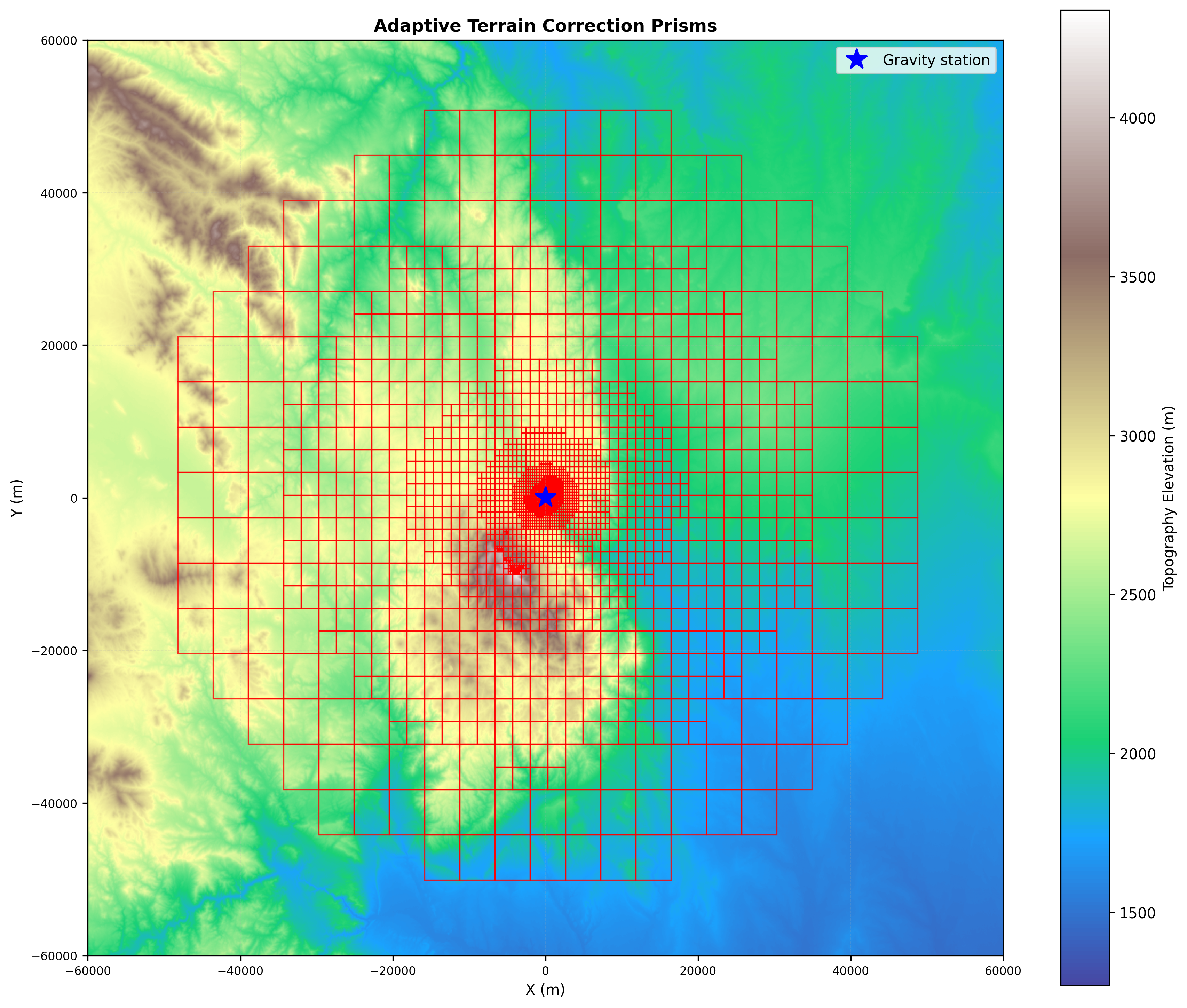
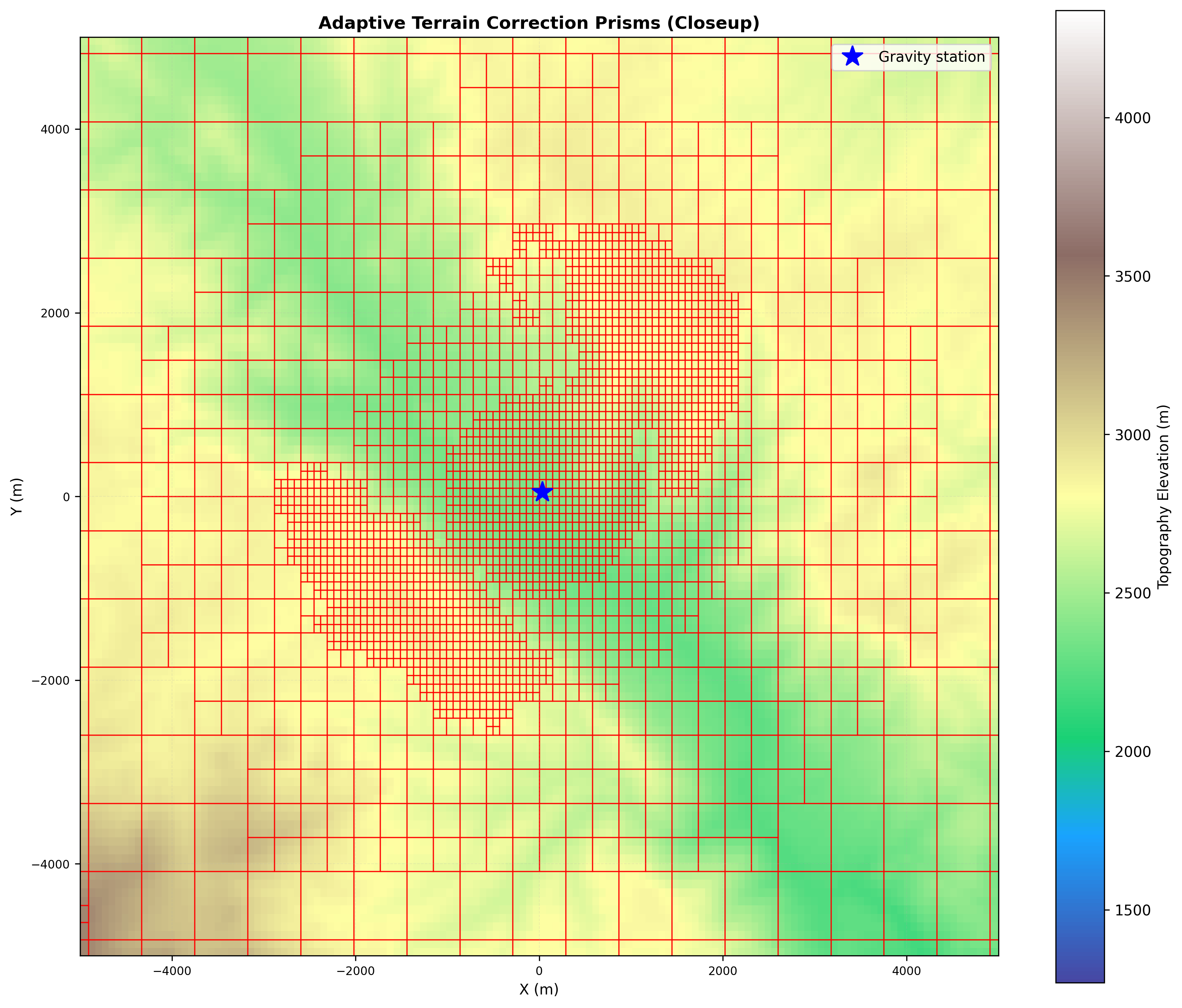
Map view of the prisms used for a terrain correction calculation for a gravity station located near Pike's Peak in Colorado, USA. The maps demonstrate how the lateral size of prisms is generally small near the station and larger further away. However, at locations with high relief relative to the station and distance, prisms with locally smaller lateral size are present. Topography data from NASA (2013)

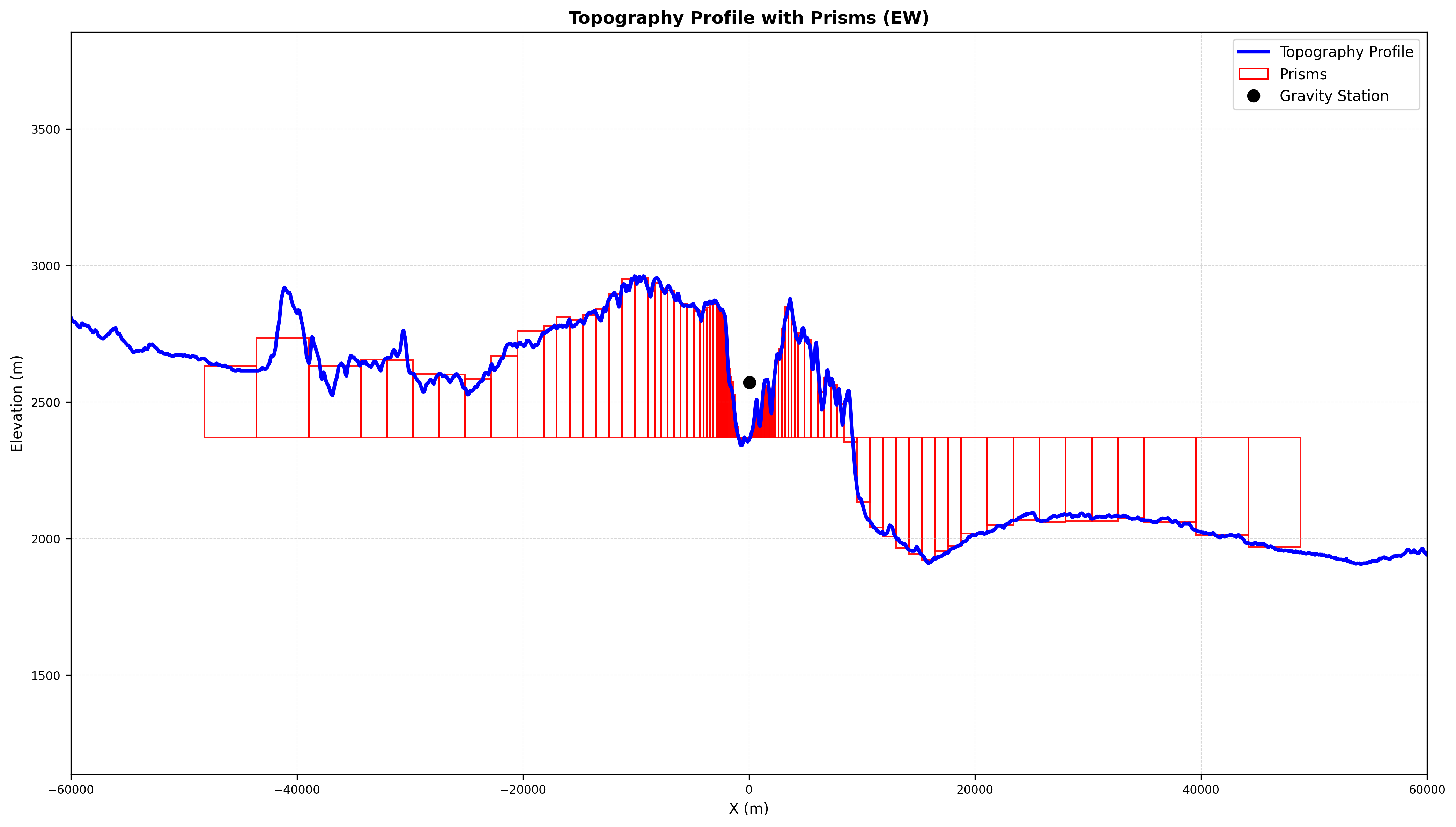
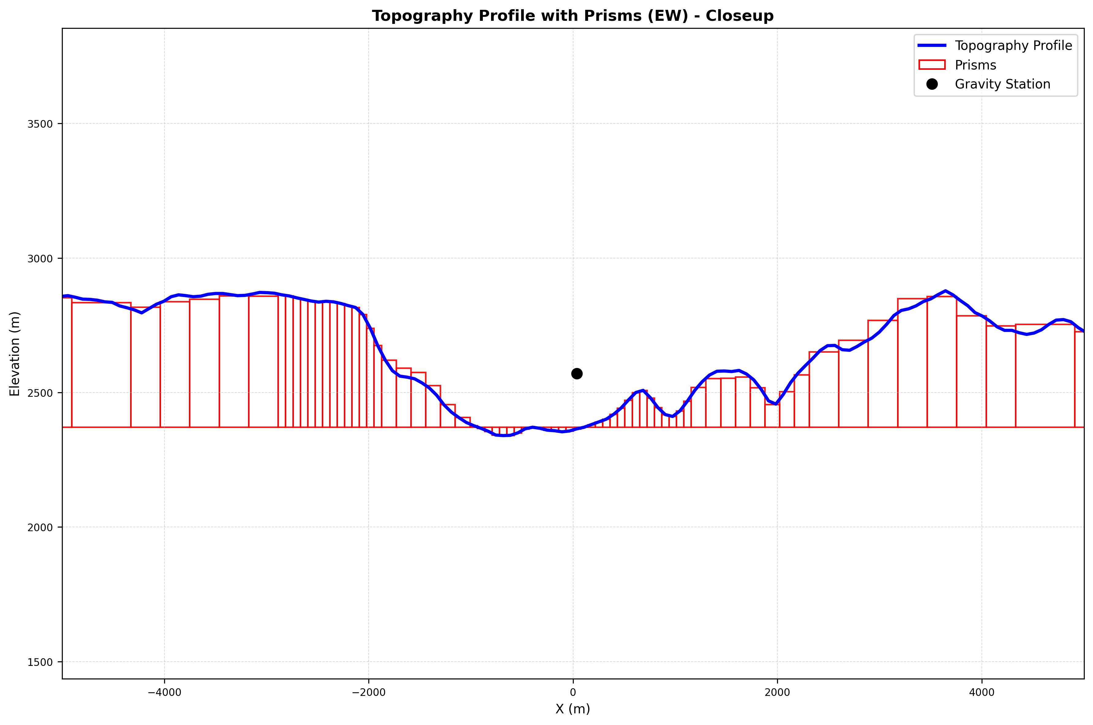
East-West profile through the aforementioned gravity station, illustrating the vertical extent of the prisms. The vertical profile similarly shows how smaller prisms are generally formed near the gravity station or at areas of high relief relative to the station. Note the high vertical exaggeration; the criterion for refining a prism depends on its longest side in either x, y, or z direction, respectively.

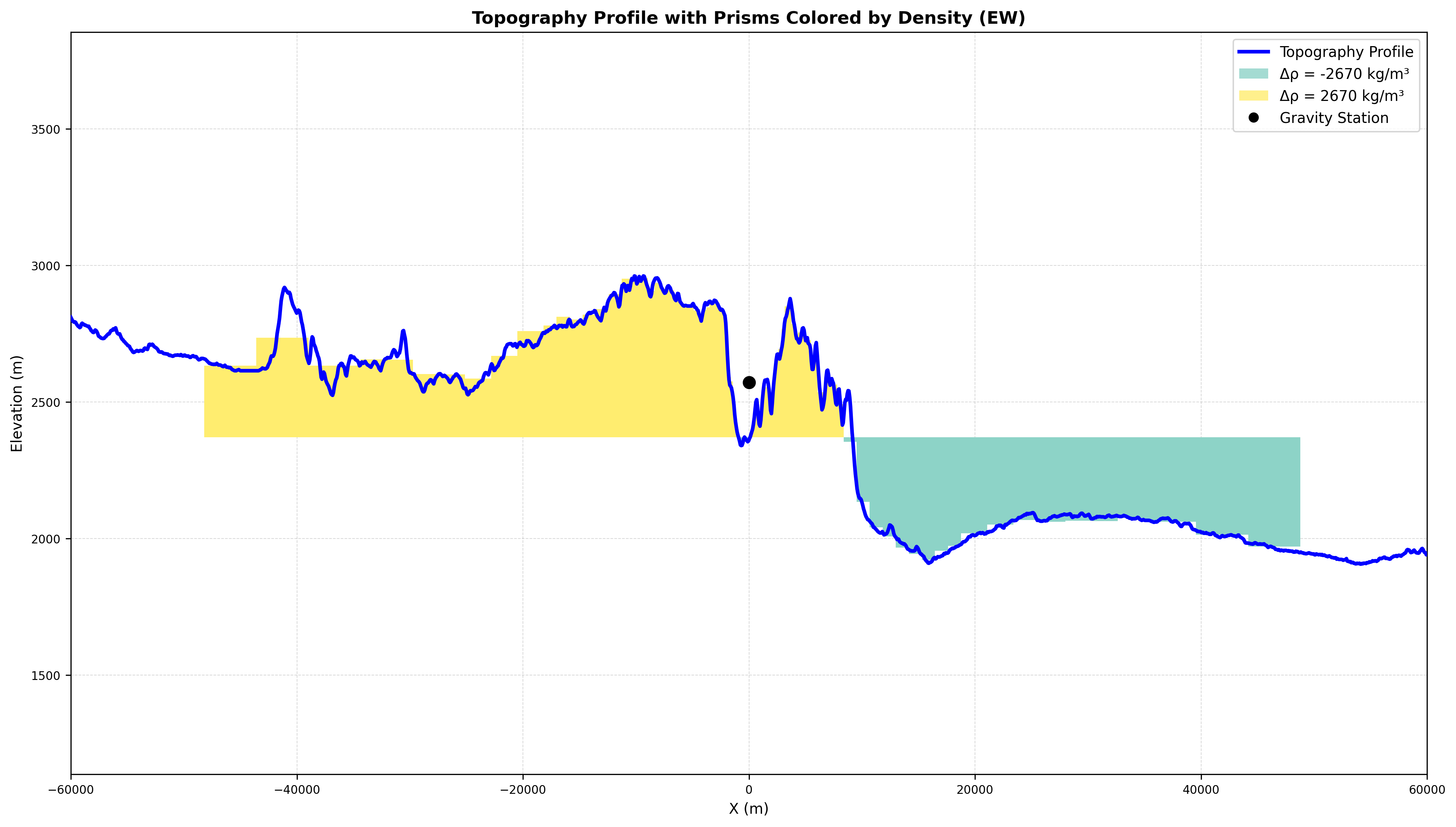
Large-scale cross-section as above, but colored by density of each prism. The terrain layer has a density of 2670 kg/m³, which contributes with opposite signs depending on whether terrain is above or below the terrain at the station location.

The adaptive approach refines prisms based on their longest side in either x, y, or z direction, respectively. The discretization strategy ensures both accuracy near the station and computational efficiency for distant terrain. This allows the ETCS to handle large datasets with high-resolution terrain grids and a large number of gravity stations while maintaining reasonable computation times. An example of such a calculation is shown in the figure below.

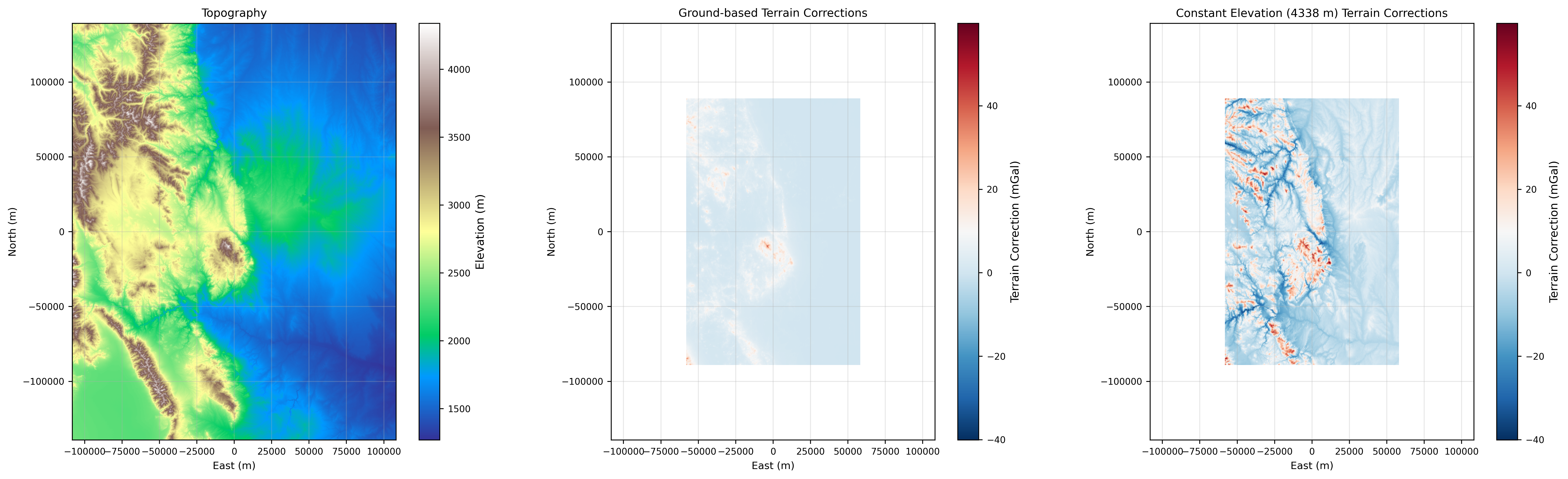
Example of multiple terrain corrections calculated for the area surrounding the example station. Left panel shows the topography (SRTM3) of the area (Pike's Peak in the center). Middle panel shows the terrain corrections calculated from the ETCS at 400,000 stations located at ground level, and right panel shows terrain corrections for airborne stations, all assumed to be located at a constant elevation of 4438 m. In both cases, a correction radius of 50 km and terrain density of 2670 kg/m³ have been assumed. Topography data is from NASA (2013) and Bathymetry from Tozer et al. (2019).

Two-layer terrain correction

The ETCS supports cases where water masses in the survey area are expected to affect gravity readings. Such cases might include marine gravity surveys in the vicinity of seafloor bathymetry and/or surveys in the vicinity of major lakes with known depth and sufficient volume that the difference between terrain and water densities should be accounted for. The ETCS employs a generalized formulation where terrain correction is treated as a process that involves two layers defined by two stratigraphic surfaces: 1) the mandatory terrain surface, which can be regarded as the top of a layer with the input (mandatory) terrain density, and 2) an optional water surface, which describes the top of a layer with the (optional) input water density. For locations without any water, the water surface is identical to the terrain surface.

The ETCS handles any survey setup that can be represented with the aforementioned two-layer model. For example, a ground-based survey can be integrated with a marine survey, a marine survey can be corrected for both subsea terrain and adjacent onshore terrain and water bodies.

As with single-layer terrain correction, the ETCS for two-layer terrain similarly employs an adaptive discretization approach. Prisms are generally refined near a gravity station and become coarser with increasing distance. In the generalized two-layer terrain situation, there are multiple ways the terrain stratigraphy can differ from the neighboring stratigraphy. The generalized approach of the ETCS acts to approximate a situation where all neighboring terrain stratigraphy is leveled to match the stratigraphy at the station. This can be illustrated in the following examples:

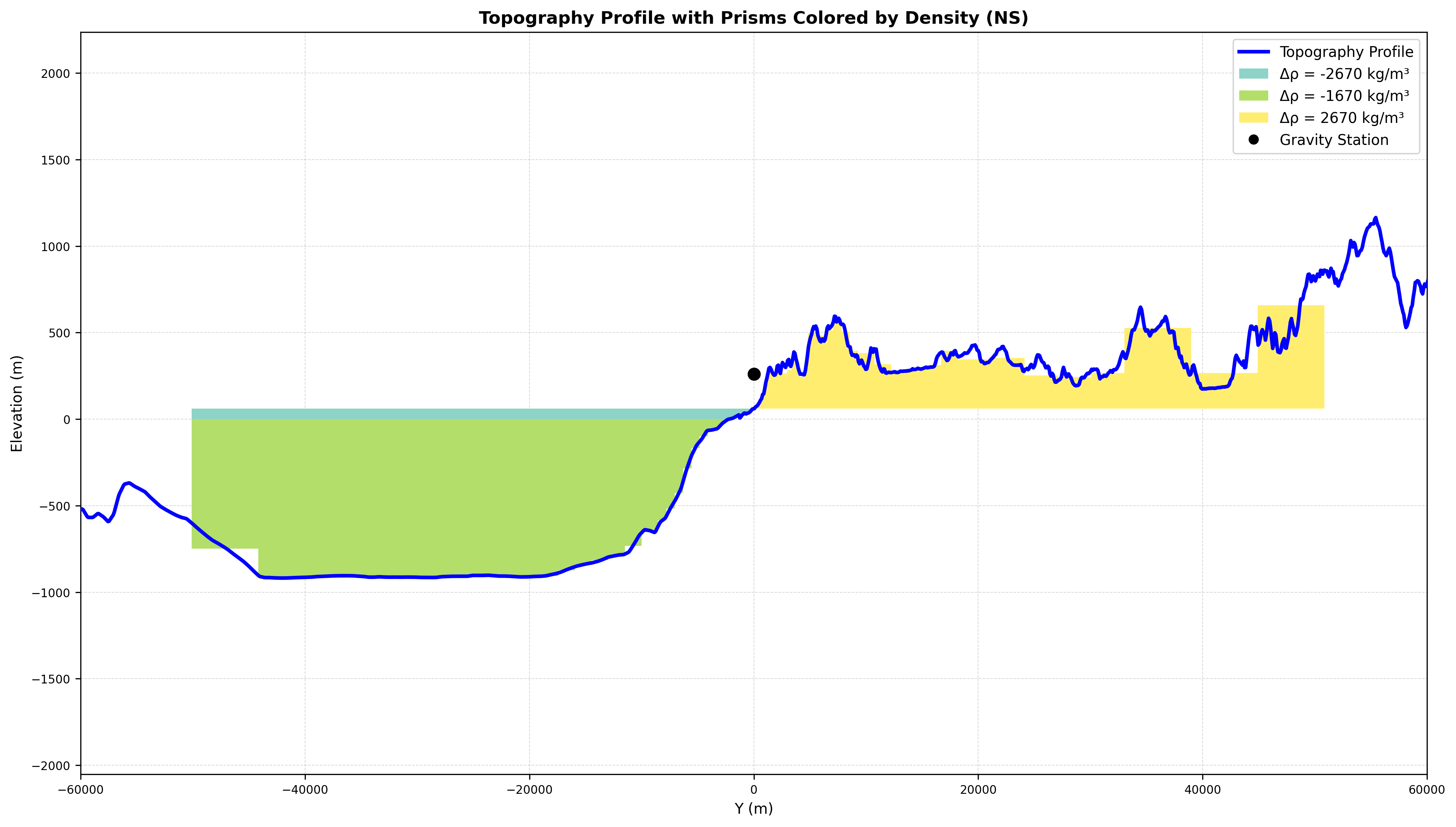
Station located above onshore terrain near a deep body of water. The ETCS represents neighboring terrain above the station terrain as material with a density of 2670 kg/m³. A neighboring column where water is present is modeled such that the water column between seafloor and sea surface is replaced with terrain. The corresponding density contrast amounts to 1000 kg/m³ − 2670 kg/m³. The "air" column between water surface and station terrain level is represented by material with a density of −2670 kg/m³.

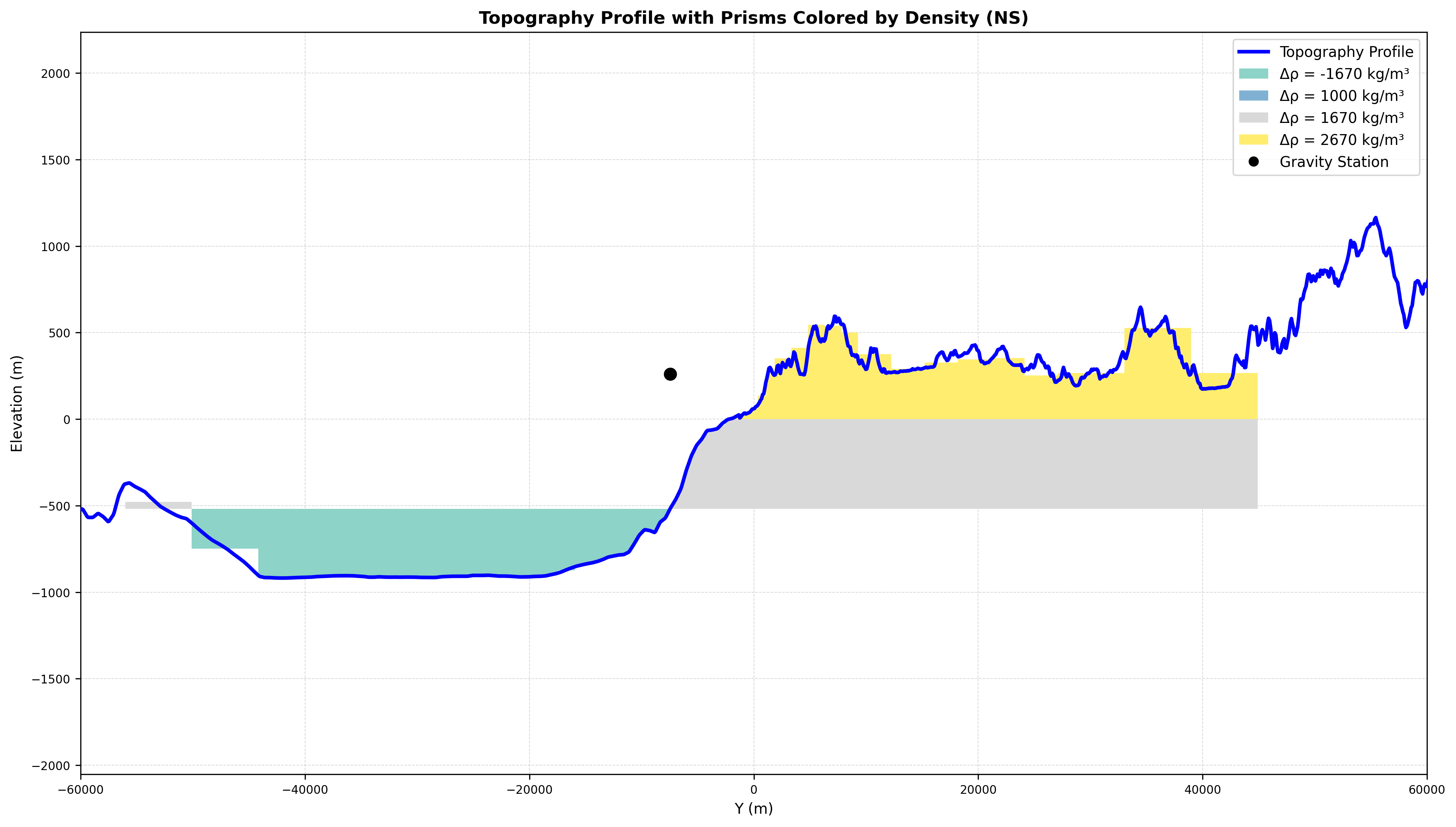
Situation where station is on or above water. The neighboring volumes with −1670 kg/m³ correction density correspond to neighboring terrain below station bathymetry where water is replaced by terrain. The volumes with 1670 kg/m³ correction density correspond to terrain above station bathymetry where terrain is replaced by water. Finally, the terrain that is both above station bathymetry and above station water level (here at z=0 m) corresponds to replacing terrain material with "air" (i.e., a density of 2670 kg/m³).

The example above is based on terrain and bathymetry surrounding the Southern California Bight coastline between Santa Barbara and Los Angeles. A map of terrain corrections in the area is shown below:

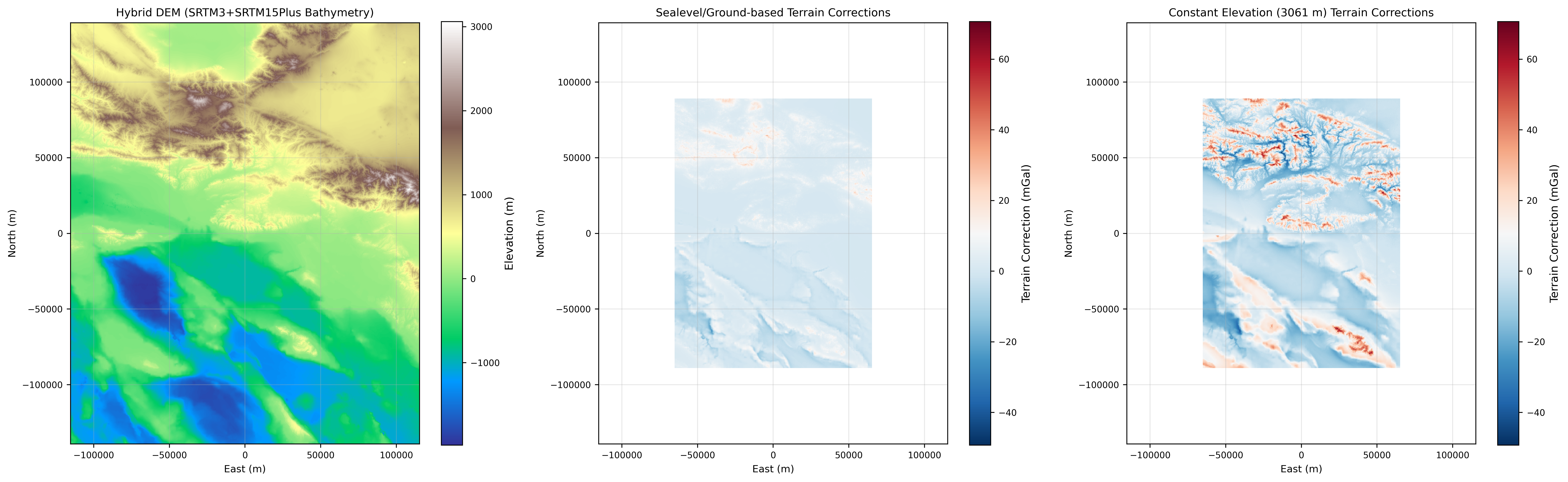
Example of multiple terrain corrections calculated for the area surrounding the example station. Left panel shows the topography (SRTM3) of the area (Southern California Bight coastline between Santa Barbara and Los Angeles). Middle panel shows the terrain corrections calculated from the ETCS at 400,000 stations located at ground level, and the right panel shows terrain corrections for airborne stations, all assumed to be located at a constant elevation of 3161 m. In both cases, a correction radius of 50 km has been assumed.

This approach can integrate any survey setup representable with the two-layer model, including combined ground-based and marine surveys, or marine surveys accounting for both subsea terrain and adjacent onshore terrain and water bodies.

Performance

The service is highly optimized and handles large datasets efficiently due to the adaptive discretization approach. Even for large terrain grid sizes (e.g., 15,000 × 15,000 grid cells) and a large number of gravity stations (e.g., 100,000 points), calculations typically complete in less than 5 minutes.

The calculation processes observation points in chunks to efficiently handle large datasets while maintaining accuracy within the specified correction radius.

Comparison with other methods

Due to adaptive discretization and floating-point precision, small numerical differences may appear at the microgal level when compared to other implementations. These differences reflect geometric modeling assumptions rather than computational inconsistencies. Importantly, the ETCS differs from the existing TC offered by Oasis Montaj (OM) which calculates TC for a square domain rather than a circular one as is the case for the ETCS. Also, the OM TC methods smoothen the topography used for calculations. The ETCS employs the topography grid 'as-is', assuming piecewise constant topography, corresponding to grid cells. This allows calculation of TC near steep terrain, e.g. vertical cliffs.

Example

For more information, see the [gravity terrain correction][gravity-terrain-correction-api-ref] API reference.

References

NASA Shuttle Radar Topography Mission (SRTM) (2013). Shuttle Radar Topography Mission (SRTM) Global. Distributed by OpenTopography. https://doi.org/10.5069/G9445JDF. Accessed: 2026-02-14.

Nowell, D. A. G. "Gravity terrain corrections—an overview." Journal of Applied Geophysics 42.2 (1999): 117-134. https://doi.org/10.1016/S0926-9851(99)00028-2.

Tozer, B, Sandwell, D. T., Smith, W. H. F., Olson, C., Beale, J. R., & Wessel, P. (2019). Global bathymetry and topography at 15 arc sec: SRTM15+. Distributed by OpenTopography. https://doi.org/10.5069/G92R3PT9. Accessed 2026-02-14

NASA Shuttle Radar Topography Mission (SRTM)(2013). Shuttle Radar Topography Mission (SRTM) Global. Distributed by OpenTopography. https://doi.org/10.5069/G9445JDF. Accessed 2026-02-14